Note
Go to the end to download the full example code.
MeshConvergence#
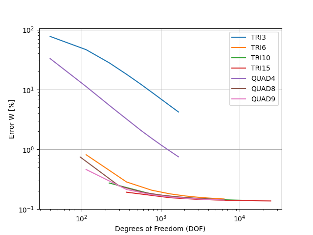
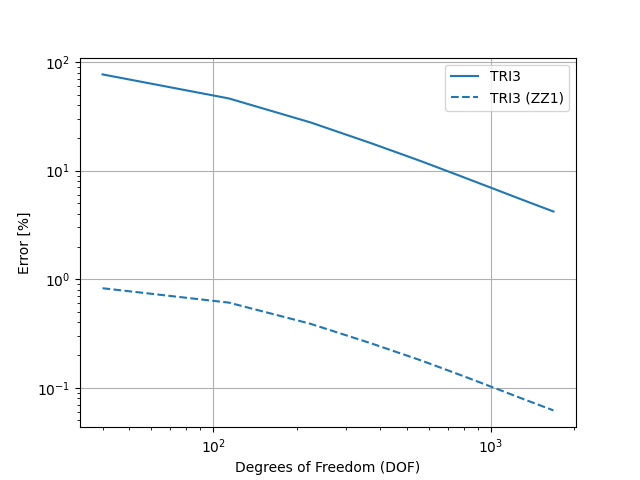
Verification of energy convergence for a bending beam for all available elements.
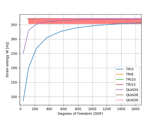

Elem: TRI3, nby:  1, Wdef = 85.307, error = 7.71e-01
Elem: TRI3, nby:  2, Wdef = 199.836, error = 4.63e-01
Elem: TRI3, nby:  3, Wdef = 268.382, error = 2.79e-01
Elem: TRI3, nby:  4, Wdef = 305.294, error = 1.79e-01
Elem: TRI3, nby:  5, Wdef = 326.756, error = 1.22e-01
Elem: TRI3, nby:  6, Wdef = 339.109, error = 8.85e-02
Elem: TRI3, nby:  7, Wdef = 347.06, error = 6.71e-02
Elem: TRI3, nby:  8, Wdef = 352.445, error = 5.26e-02
Elem: TRI3, nby:  9, Wdef = 356.373, error = 4.21e-02
Elem: TRI6, nby:  1, Wdef = 369.006, error = 8.10e-03
Elem: TRI6, nby:  2, Wdef = 370.965, error = 2.84e-03
Elem: TRI6, nby:  3, Wdef = 371.253, error = 2.06e-03
Elem: TRI6, nby:  4, Wdef = 371.354, error = 1.79e-03
Elem: TRI6, nby:  5, Wdef = 371.405, error = 1.65e-03
Elem: TRI6, nby:  6, Wdef = 371.433, error = 1.58e-03
Elem: TRI6, nby:  7, Wdef = 371.451, error = 1.53e-03
Elem: TRI6, nby:  8, Wdef = 371.463, error = 1.50e-03
Elem: TRI6, nby:  9, Wdef = 371.472, error = 1.47e-03
Elem: TRI10, nby:  1, Wdef = 371.008, error = 2.72e-03
Elem: TRI10, nby:  2, Wdef = 371.36, error = 1.78e-03
Elem: TRI10, nby:  3, Wdef = 371.433, error = 1.58e-03
Elem: TRI10, nby:  4, Wdef = 371.463, error = 1.50e-03
Elem: TRI10, nby:  5, Wdef = 371.479, error = 1.45e-03
Elem: TRI10, nby:  6, Wdef = 371.489, error = 1.43e-03
Elem: TRI10, nby:  7, Wdef = 371.495, error = 1.41e-03
Elem: TRI10, nby:  8, Wdef = 371.499, error = 1.40e-03
Elem: TRI10, nby:  9, Wdef = 371.503, error = 1.39e-03
Elem: TRI15, nby:  1, Wdef = 371.309, error = 1.91e-03
Elem: TRI15, nby:  2, Wdef = 371.445, error = 1.55e-03
Elem: TRI15, nby:  3, Wdef = 371.478, error = 1.46e-03
Elem: TRI15, nby:  4, Wdef = 371.493, error = 1.42e-03
Elem: TRI15, nby:  5, Wdef = 371.501, error = 1.40e-03
Elem: TRI15, nby:  6, Wdef = 371.505, error = 1.39e-03
Elem: TRI15, nby:  7, Wdef = 371.508, error = 1.38e-03
Elem: TRI15, nby:  8, Wdef = 371.511, error = 1.37e-03
Elem: TRI15, nby:  9, Wdef = 371.512, error = 1.37e-03
Elem: QUAD4, nby:  1, Wdef = 249.865, error = 3.28e-01
Elem: QUAD4, nby:  2, Wdef = 330.381, error = 1.12e-01
Elem: QUAD4, nby:  3, Wdef = 351.849, error = 5.42e-02
Elem: QUAD4, nby:  4, Wdef = 360.11, error = 3.20e-02
Elem: QUAD4, nby:  5, Wdef = 364.354, error = 2.06e-02
Elem: QUAD4, nby:  6, Wdef = 366.455, error = 1.50e-02
Elem: QUAD4, nby:  7, Wdef = 367.75, error = 1.15e-02
Elem: QUAD4, nby:  8, Wdef = 368.603, error = 9.19e-03
Elem: QUAD4, nby:  9, Wdef = 369.241, error = 7.47e-03
Elem: QUAD8, nby:  1, Wdef = 369.262, error = 7.42e-03
Elem: QUAD8, nby:  2, Wdef = 371.115, error = 2.43e-03
Elem: QUAD8, nby:  3, Wdef = 371.315, error = 1.90e-03
Elem: QUAD8, nby:  4, Wdef = 371.386, error = 1.70e-03
Elem: QUAD8, nby:  5, Wdef = 371.424, error = 1.60e-03
Elem: QUAD8, nby:  6, Wdef = 371.445, error = 1.55e-03
Elem: QUAD8, nby:  7, Wdef = 371.46, error = 1.51e-03
Elem: QUAD8, nby:  8, Wdef = 371.47, error = 1.48e-03
Elem: QUAD8, nby:  9, Wdef = 371.478, error = 1.46e-03
Elem: QUAD9, nby:  1, Wdef = 370.315, error = 4.58e-03
Elem: QUAD9, nby:  2, Wdef = 371.231, error = 2.12e-03
Elem: QUAD9, nby:  3, Wdef = 371.375, error = 1.74e-03
Elem: QUAD9, nby:  4, Wdef = 371.428, error = 1.59e-03
Elem: QUAD9, nby:  5, Wdef = 371.456, error = 1.52e-03
Elem: QUAD9, nby:  6, Wdef = 371.471, error = 1.48e-03
Elem: QUAD9, nby:  7, Wdef = 371.481, error = 1.45e-03
Elem: QUAD9, nby:  8, Wdef = 371.488, error = 1.43e-03
Elem: QUAD9, nby:  9, Wdef = 371.494, error = 1.42e-03

WSA = 372.0206 mJ

Mesh: 1.143 s
Boundary Conditions: 1.036 ms
Matrix: 1.644 s
Solver: 1.004 s
Resolutions: 2.173 s
PostProcessing: 278.500 ms
Display: 1.166 s
13 import matplotlib.pyplot as plt
14 import numpy as np
15
16 from EasyFEA import Display, Folder, Models, Tic, ElemType, Simulations, Paraview
17 from EasyFEA.Geoms import Domain, Point
18
19 if __name__ == "__main__":
20 Display.Clear()
21
22 # ----------------------------------------------
23 # Configuration
24 # ----------------------------------------------
25 dim = 2 # Define the dimension of the problem (2D or 3D)
26
27 # outputs
28 folder = Folder.Results_Dir() + f"{dim}D"
29 plotResult = True
30 makeParaview = False
31
32 # geom
33 L = 120 # mm
34 h = 13 # Height
35 b = 13 # Width
36
37 # model
38 E = 210000 # MPa (Young's modulus)
39 v = 0.25 # Poisson's ratio
40 material = Models.Elastic.Isotropic(dim, thickness=b, E=E, v=v, planeStress=True)
41
42 # load
43 P = 800 # N
44
45 # expected energy
46 WdefRef = 2 * P**2 * L / E / h / b * (L**2 / h / b + (1 + v) * 3 / 5)
47
48 # ----------------------------------------------
49 # Mesh
50 # ----------------------------------------------
51 isOrganised = True
52
53 # List of mesh sizes (number of elements) to investigate convergence
54 if dim == 2:
55 list_N = np.arange(1, 10, 1)
56 else:
57 list_N = np.arange(1, 8, 2)
58
59 # Lists to store data for plotting
60 times_elem_N = [] # times for element type and N size
61 wDef_elem_N = [] # energy
62 dofs_elem_N = [] # dofs
63 zz1_elem_N = [] # zz1
64
65 # ----------------------------------------------
66 # Simulations
67 # ----------------------------------------------
68
69 # Loop over each element type for both 2D and 3D simulations
70 elemTypes = ElemType.Get_2D()[:] if dim == 2 else ElemType.Get_3D()
71
72 # elemTypes = [elem.name for elem in elemTypes.copy()]
73
74 for e, elemType in enumerate(elemTypes):
75 times_N = []
76 wDef_N = []
77 dofs_N = []
78 zz1_N = []
79
80 # Loop over each mesh size (number of elements)
81 for N in list_N:
82 meshSize = b / N
83
84 # Define the domain for the mesh
85 domain = Domain(Point(), Point(x=L, y=h), meshSize)
86
87 # Generate the mesh using Gmsh
88 if dim == 2:
89 mesh = domain.Mesh_2D([], elemType, isOrganised=isOrganised)
90 volume = mesh.area * material.thickness
91 else:
92 mesh = domain.Mesh_Extrude(
93 [],
94 elemType=elemType,
95 extrude=[0, 0, b],
96 layers=[4],
97 isOrganised=isOrganised,
98 )
99 volume = mesh.volume
100 # Ensure that the volume matches the expected value (L * h * b)
101 assert np.abs(volume - (L * h * b)) / volume <= 1e-10
102
103 # Define nodes on the left boundary (x=0) and right boundary (x=L)
104 nodes_x0 = mesh.Nodes_Conditions(lambda x, y, z: x == 0)
105 nodes_xL = mesh.Nodes_Conditions(lambda x, y, z: x == L)
106
107 # Create or update the simulation object with the current mesh
108 if e == 0 and N == list_N[0]:
109 simu = Simulations.Elastic(mesh, material)
110 else:
111 simu.Bc_Init()
112 simu.mesh = mesh
113
114 # Set displacement boundary conditions
115 simu.add_dirichlet(nodes_x0, [0] * dim, simu.Get_unknowns())
116 # Set surface load on the right boundary (y-direction)
117 simu.add_surfLoad(nodes_xL, [-P / h / b], ["y"])
118
119 tic = Tic()
120
121 # Solve the simulation
122 simu.Solve()
123 simu.Save_Iter()
124
125 time = tic.Tac("Resolutions", "Total time", False)
126
127 # Get the computed deformation energy
128 Wdef = simu.Result("Wdef")
129
130 # Store the results for the current mesh size
131 times_N.append(time)
132 wDef_N.append(Wdef)
133 dofs_N.append(mesh.Nn * dim)
134 zz1_N.append(simu.Result("ZZ1"))
135
136 if elemType != mesh.elemType:
137 print("Error in mesh generation")
138
139 print(
140 f"Elem: {mesh.elemType}, nby: {N:2}, Wdef = {np.round(Wdef, 3)}, "
141 f"error = {np.abs(WdefRef - Wdef) / WdefRef:.2e}"
142 )
143
144 # Store the results for the current element type
145 times_elem_N.append(times_N)
146 wDef_elem_N.append(wDef_N)
147 dofs_elem_N.append(dofs_N)
148 zz1_elem_N.append(zz1_N)
149
150 # ----------------------------------------------
151 # Results
152 # ----------------------------------------------
153 # Display the convergence of deformation energy
154 ax_Wdef = Display.Init_Axes()
155 ax_error = Display.Init_Axes()
156 ax_times = Display.Init_Axes()
157 ax_zz1 = Display.Init_Axes()
158
159 print(f"\nWSA = {np.round(WdefRef, 4)} mJ")
160
161 for e, elemType in enumerate(elemTypes):
162 # Convergence of deformation energy
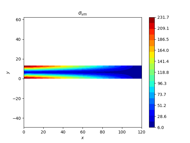
163 ax_Wdef.plot(dofs_elem_N[e], wDef_elem_N[e])
164
165 # Error in deformation energy
166 Wdef = np.array(wDef_elem_N[e])
167 error = (WdefRef - Wdef) / WdefRef * 100
168 ax_error.loglog(dofs_elem_N[e], error)
169
170 # Computation time
171 ax_times.loglog(dofs_elem_N[e], times_elem_N[e])
172 # ax_Times.plot(listDofs_e_nb[e], listTimes_e_nb[e])
173 # ax_Times.set_xscale('log')
174
175 # ZZ1
176 if elemType == elemTypes[0]:
177 last = ax_zz1.loglog(dofs_elem_N[e], error, label=f"{elemType}")
178 ax_zz1.loglog(
179 dofs_elem_N[e],
180 zz1_elem_N[e],
181 ls="--",
182 color=last[0]._color,
183 label=f"{elemType} (ZZ1)",
184 )
185
186 WdefRefArray = np.ones_like(dofs_elem_N[0]) * WdefRef
187 WdefRefArray5 = WdefRefArray * 0.95
188 # WdefRefArray5 = WdefRefArray * 1
189
190 # Deformation energy
191 ax_Wdef.grid()
192 ax_Wdef.set_xlim([-10, np.max(dofs_elem_N[0])])
193 ax_Wdef.set_xlabel("Degrees of Freedom (DOF)")
194 ax_Wdef.set_ylabel("Strain energy W [mJ]")
195 ax_Wdef.legend(elemTypes)
196 # ax_Wdef.fill_between(dofs_N, WdefRefArray, WdefRefArray5, alpha=0.5, color='red')
197 ax_Wdef.fill_between(dofs_N, WdefRefArray, WdefRefArray5, alpha=0.5, color="red")
198 plt.figure(ax_Wdef.figure)
199 Display.Save_fig(folder, "Energy")
200
201 # Error in deformation energy
202 ax_error.grid()
203 ax_error.set_xlabel("Degrees of Freedom (DOF)")
204 ax_error.set_ylabel("Error W [%]")
205 ax_error.legend(elemTypes)
206 plt.figure(ax_error.figure)
207 Display.Save_fig(folder, "Error")
208
209 # Error in deformation energy
210 ax_zz1.grid()
211 ax_zz1.set_xlabel("Degrees of Freedom (DOF)")
212 ax_zz1.set_ylabel("Error [%]")
213 ax_zz1.legend()
214 plt.figure(ax_zz1.figure)
215 Display.Save_fig(folder, "Error ZZ1")
216
217 # Computation time
218 ax_times.grid()
219 ax_times.set_xlabel("Degrees of Freedom (DOF)")
220 ax_times.set_ylabel("Computation Time [s]")
221 ax_times.legend(elemTypes)
222 plt.figure(ax_times.figure)
223 Display.Save_fig(folder, "Time")
224
225 # Plot the von Mises stress result using 20 color levels
226 Display.Plot_Result(simu, "Svm", ncolors=20)
227
228 if makeParaview:
229 # Generate Paraview files for visualization
230 Paraview.Save_simu(simu, folder, details=True)
231
232 # Show the total computation time
233 print()
234 Tic.Resume()
235
236 # Display the computation time history
237 # Tic.Plot_History(folder)
238
239 # Show all plots
240 plt.show()
Total running time of the script: (0 minutes 5.435 seconds)