Note
Go to the end to download the full example code.
Beam3#
A bi-fixed beam undergoing bending deformation.
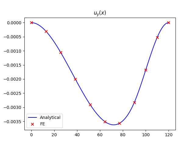
err uy: 1.27e-12%
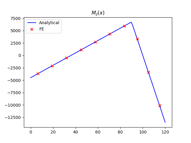
err Mz : 1.19e-12 %
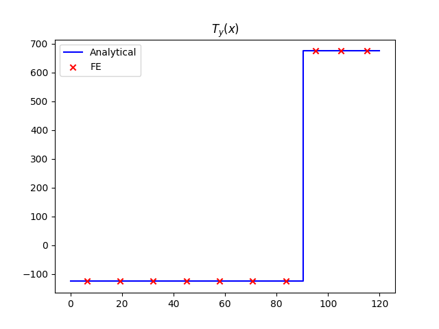
err Ty : 2.21e-12 %
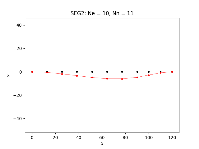
==================== Mesh ====================
Element type: SEG2
Ne = 10, Nn = 11
==================== Model ====================
<EasyFEA.Models.Beam._beam.BeamStructure object at 0x74224465bc50>
solver:scipy
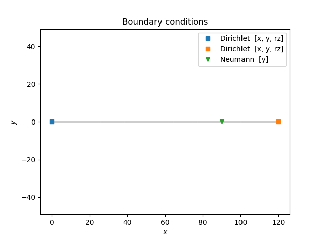
============= Boundary Conditions =============
Unspecified.
=================== Results ===================
Ux max = 0.00e+00
Ux min = 0.00e+00
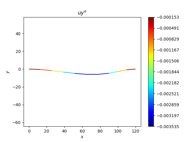
Uy max = 0.00e+00
Uy min = -3.56e-03
=================== TicTac ===================
Mesh: 67.945 ms
Boundary Conditions: 20.027 µs
Matrix: 18.277 ms
Solver: 1.110 ms
Display: 62.850 ms
13 import matplotlib.pyplot as plt
14 import numpy as np
15
16 from EasyFEA import Display, Models, Mesher, ElemType, Simulations
17 from EasyFEA.Geoms import Line, Point, Points
18
19 if __name__ == "__main__":
20 Display.Clear()
21
22 # ----------------------------------------------
23 # Configuration
24 # ----------------------------------------------
25
26 # geom
27 L = 120
28 h = 20
29 b = 13
30 e = 2
31
32 # model
33 E = 210000
34 v = 0.3
35 useTimoshenko = False
36
37 # load
38 F = -800
39
40 # ----------------------------------------------
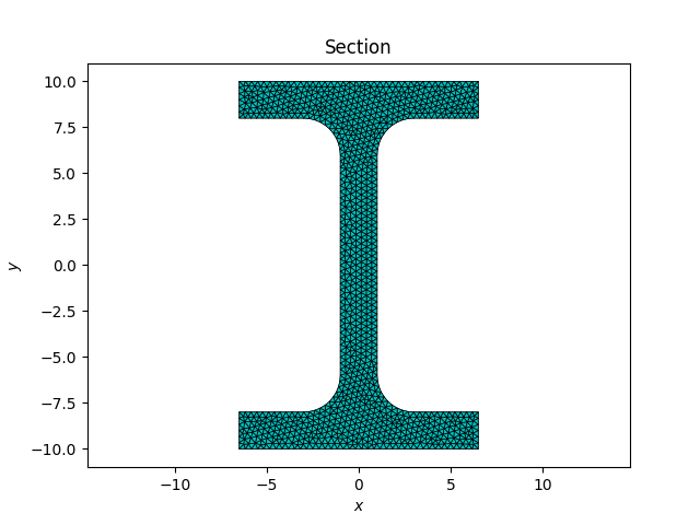
41 # Section
42 # ----------------------------------------------
43
44 def DoSym(p: Point, n: np.ndarray) -> Point:
45 pc = p.copy()
46 pc.Symmetry(n=n)
47 return pc
48
49 p1 = Point(-b / 2, -h / 2)
50 p2 = Point(b / 2, -h / 2)
51 p3 = Point(b / 2, -h / 2 + e)
52 p4 = Point(e / 2, -h / 2 + e, r=e)
53 p5 = DoSym(p4, (0, 1))
54 p6 = DoSym(p3, (0, 1))
55 p7 = DoSym(p2, (0, 1))
56 p8 = DoSym(p1, (0, 1))
57 p9 = DoSym(p6, (1, 0))
58 p10 = DoSym(p5, (1, 0))
59 p11 = DoSym(p4, (1, 0))
60 p12 = DoSym(p3, (1, 0))
61 contour = Points([p1, p2, p3, p4, p5, p6, p7, p8, p9, p10, p11, p12], e / 6)
62 section = Mesher().Mesh_2D(contour)
63
64 # ----------------------------------------------
65 # Mesh
66 # ----------------------------------------------
67
68 elemType = ElemType.SEG2
69 beamDim = 2 # must be >= 2
70
71 p1 = Point()
72 pL = Point(x=L * 0.75)
73 p2 = Point(x=L)
74 line = Line(p1, p2, L / 9)
75 beam = Models.Beam.Isotropic(beamDim, line, section, E, v)
76
77 mesh = Mesher().Mesh_Beams([beam], additionalPoints=[pL], elemType=elemType)
78
79 # ----------------------------------------------
80 # Simulation
81 # ----------------------------------------------
82
83 # Initialize the beam structure with the defined beam segments
84 beamStructure = Models.Beam.BeamStructure([beam])
85
86 # Create the beam simulation
87 simu = Simulations.Beam(mesh, beamStructure, useTimoshenko=useTimoshenko)
88 dof_n = simu.Get_dof_n()
89
90 # Apply boundary conditions
91 simu.add_dirichlet(mesh.Nodes_Point(p1), [0] * dof_n, simu.Get_unknowns())
92 simu.add_dirichlet(mesh.Nodes_Point(p2), [0] * dof_n, simu.Get_unknowns())
93 simu.add_neumann(mesh.Nodes_Point(pL), [F], ["y"])
94
95 # Solve the beam problem and get displacement results
96 sol = simu.Solve()
97 simu.Save_Iter()
98
99 # ----------------------------------------------
100 # Results
101 # ----------------------------------------------
102
103 Display.Plot_Mesh(simu, L / 20 / sol.min())
104 ax = Display.Plot_Mesh(section)
105 ax.set_title("Section")
106 Display.Plot_BoundaryConditions(simu)
107 Display.Plot_Result(simu, "uy", L / 20 / sol.min())
108
109 # ------------------------
110 # uy
111 # ------------------------
112
113 # beam properties
114 Iz = beam.Iz
115 G = beam.mu
116 A = section.area
117
118 # general reactions and fixed-end moment (valid for arbitrary pL.x)
119 a = pL.x
120 b = L - a
121 Ra = -F * b**2 * (3 * a + b) / L**3 # upward reaction at x=0
122 Rb = -F * a**2 * (a + 3 * b) / L**3 # upward reaction at x=L
123 Ma = F * a * b**2 / L**2 # fixed-end moment at x=0
124
125 x = np.linspace(0, L, 100)
126 x_n = mesh.coord[:, 0]
127 x_e = x_n[mesh.connect].mean(1) # element centroid x-coords
128
129 def uy_x(x):
130 x = np.asarray(x)
131 macaulay = np.where(x > a, (x - a) ** 3 / 6, 0.0)
132 return (Ma / 2 * x**2 + Ra / 6 * x**3 + F * macaulay) / (E * Iz)
133
134 uy = simu.Result("uy")
135 err_uy = np.abs(uy_x(x_n) - uy).max() / np.abs(uy_x(a))
136 Display.MyPrint(f"\nerr uy: {err_uy * 100:.2e}%")
137
138 ax_uy = Display.Init_Axes()
139 ax_uy.plot(x, uy_x(x), label="Analytical", c="blue")
140 ax_uy.scatter(x_n, uy, label="FE", c="red", marker="x", zorder=2)
141 ax_uy.set_title("$u_y(x)$")
142 ax_uy.legend()
143
144 # ------------------------
145 # Mz
146 # ------------------------
147
148 def Mz_x(x):
149 x = np.asarray(x)
150 Ma_plus_Ra_x = Ma + Ra * x
151 return np.where(x <= a, Ma_plus_Ra_x, Ma_plus_Ra_x + F * (x - a))
152
153 Mz = simu.Result("Mz", nodeValues=False)
154 err_Mz = np.abs(Mz_x(x_e) - Mz).max() / np.abs(Mz_x(x_e)).max()
155 Display.MyPrint(f"\nerr Mz : {err_Mz * 100:.2e} %")
156
157 axMz = Display.Init_Axes()
158 axMz.plot(x, Mz_x(x), label="Analytical", c="blue")
159 axMz.scatter(x_e, Mz, label="FE", c="red", marker="x", zorder=2)
160 axMz.set_title("$M_z(x)$")
161 axMz.legend()
162
163 # ------------------------
164 # Ty
165 # ------------------------
166
167 def Ty_x(x):
168 x = np.asarray(x)
169 return np.where(x < a, -Ra, Rb)
170
171 Ty = simu.Result("Ty", nodeValues=False)
172 err_Ty = np.abs(Ty_x(x_e) - Ty).max() / max(Ra, Rb)
173 Display.MyPrint(f"\nerr Ty : {err_Ty * 100:.2e} %")
174
175 ax_Ty = Display.Init_Axes()
176 ax_Ty.step(x, Ty_x(x), label="Analytical", c="blue", where="mid")
177 ax_Ty.scatter(x_e, Ty, label="FE", c="red", marker="x", zorder=2)
178 ax_Ty.set_title("$T_y(x)$")
179 ax_Ty.legend()
180
181 print(simu)
182
183 plt.show()
Total running time of the script: (0 minutes 0.571 seconds)