Note
Go to the end to download the full example code.
MeshConvergence#
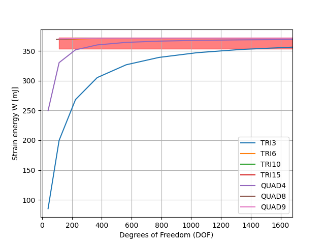
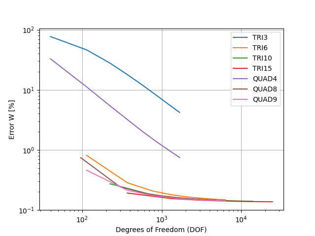
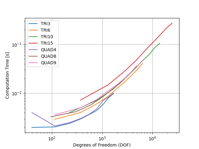
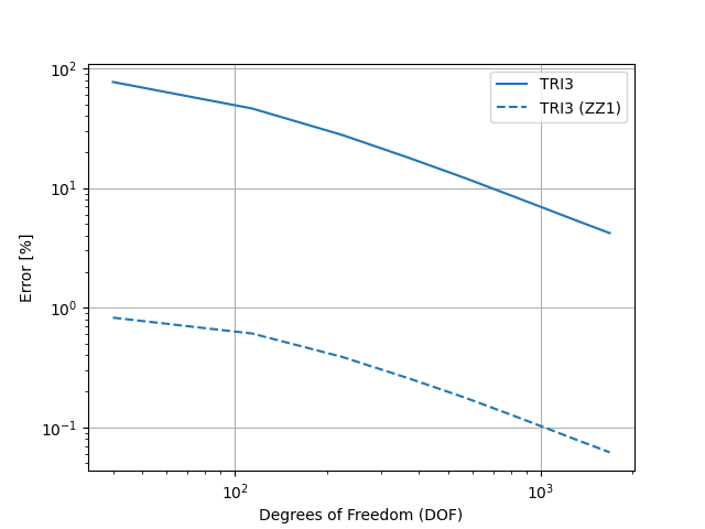
Verification of energy convergence for a bending beam for all available elements.
Elem: TRI3, nby:  1, Wdef = 85.307, error = 7.71e-01
Elem: TRI3, nby:  2, Wdef = 199.836, error = 4.63e-01
Elem: TRI3, nby:  3, Wdef = 268.382, error = 2.79e-01
Elem: TRI3, nby:  4, Wdef = 305.294, error = 1.79e-01
Elem: TRI3, nby:  5, Wdef = 326.756, error = 1.22e-01
Elem: TRI3, nby:  6, Wdef = 339.109, error = 8.85e-02
Elem: TRI3, nby:  7, Wdef = 347.06, error = 6.71e-02
Elem: TRI3, nby:  8, Wdef = 352.445, error = 5.26e-02
Elem: TRI3, nby:  9, Wdef = 356.373, error = 4.21e-02
Elem: TRI6, nby:  1, Wdef = 369.006, error = 8.10e-03
Elem: TRI6, nby:  2, Wdef = 370.965, error = 2.84e-03
Elem: TRI6, nby:  3, Wdef = 371.253, error = 2.06e-03
Elem: TRI6, nby:  4, Wdef = 371.354, error = 1.79e-03
Elem: TRI6, nby:  5, Wdef = 371.405, error = 1.65e-03
Elem: TRI6, nby:  6, Wdef = 371.433, error = 1.58e-03
Elem: TRI6, nby:  7, Wdef = 371.451, error = 1.53e-03
Elem: TRI6, nby:  8, Wdef = 371.463, error = 1.50e-03
Elem: TRI6, nby:  9, Wdef = 371.472, error = 1.47e-03
Elem: TRI10, nby:  1, Wdef = 371.008, error = 2.72e-03
Elem: TRI10, nby:  2, Wdef = 371.36, error = 1.78e-03
Elem: TRI10, nby:  3, Wdef = 371.433, error = 1.58e-03
Elem: TRI10, nby:  4, Wdef = 371.463, error = 1.50e-03
Elem: TRI10, nby:  5, Wdef = 371.479, error = 1.45e-03
Elem: TRI10, nby:  6, Wdef = 371.489, error = 1.43e-03
Elem: TRI10, nby:  7, Wdef = 371.495, error = 1.41e-03
Elem: TRI10, nby:  8, Wdef = 371.499, error = 1.40e-03
Elem: TRI10, nby:  9, Wdef = 371.503, error = 1.39e-03
Elem: TRI15, nby:  1, Wdef = 371.309, error = 1.91e-03
Elem: TRI15, nby:  2, Wdef = 371.445, error = 1.55e-03
Elem: TRI15, nby:  3, Wdef = 371.478, error = 1.46e-03
Elem: TRI15, nby:  4, Wdef = 371.493, error = 1.42e-03
Elem: TRI15, nby:  5, Wdef = 371.501, error = 1.40e-03
Elem: TRI15, nby:  6, Wdef = 371.505, error = 1.39e-03
Elem: TRI15, nby:  7, Wdef = 371.508, error = 1.38e-03
Elem: TRI15, nby:  8, Wdef = 371.511, error = 1.37e-03
Elem: TRI15, nby:  9, Wdef = 371.512, error = 1.37e-03
Elem: QUAD4, nby:  1, Wdef = 249.865, error = 3.28e-01
Elem: QUAD4, nby:  2, Wdef = 330.381, error = 1.12e-01
Elem: QUAD4, nby:  3, Wdef = 351.849, error = 5.42e-02
Elem: QUAD4, nby:  4, Wdef = 360.11, error = 3.20e-02
Elem: QUAD4, nby:  5, Wdef = 364.354, error = 2.06e-02
Elem: QUAD4, nby:  6, Wdef = 366.455, error = 1.50e-02
Elem: QUAD4, nby:  7, Wdef = 367.75, error = 1.15e-02
Elem: QUAD4, nby:  8, Wdef = 368.603, error = 9.19e-03
Elem: QUAD4, nby:  9, Wdef = 369.241, error = 7.47e-03
Elem: QUAD8, nby:  1, Wdef = 369.262, error = 7.42e-03
Elem: QUAD8, nby:  2, Wdef = 371.115, error = 2.43e-03
Elem: QUAD8, nby:  3, Wdef = 371.315, error = 1.90e-03
Elem: QUAD8, nby:  4, Wdef = 371.386, error = 1.70e-03
Elem: QUAD8, nby:  5, Wdef = 371.424, error = 1.60e-03
Elem: QUAD8, nby:  6, Wdef = 371.445, error = 1.55e-03
Elem: QUAD8, nby:  7, Wdef = 371.46, error = 1.51e-03
Elem: QUAD8, nby:  8, Wdef = 371.47, error = 1.48e-03
Elem: QUAD8, nby:  9, Wdef = 371.478, error = 1.46e-03
Elem: QUAD9, nby:  1, Wdef = 370.315, error = 4.58e-03
Elem: QUAD9, nby:  2, Wdef = 371.231, error = 2.12e-03
Elem: QUAD9, nby:  3, Wdef = 371.375, error = 1.74e-03
Elem: QUAD9, nby:  4, Wdef = 371.428, error = 1.59e-03
Elem: QUAD9, nby:  5, Wdef = 371.456, error = 1.52e-03
Elem: QUAD9, nby:  6, Wdef = 371.471, error = 1.48e-03
Elem: QUAD9, nby:  7, Wdef = 371.481, error = 1.45e-03
Elem: QUAD9, nby:  8, Wdef = 371.488, error = 1.43e-03
Elem: QUAD9, nby:  9, Wdef = 371.494, error = 1.42e-03

WSA = 372.0206 mJ

Mesh : 855.425 ms
Boundary Conditions : 798.464 µs
Matrix : 1.482 s
Solver : 845.271 ms
Resolutions : 1.870 s
PostProcessing : 226.916 ms
Display : 782.873 ms
13 import matplotlib.pyplot as plt
14 import numpy as np
15
16 from EasyFEA import Display, Folder, Models, Tic, ElemType, Simulations, Paraview
17 from EasyFEA.Geoms import Domain, Point
18
19 if __name__ == "__main__":
20 Display.Clear()
21
22 # ----------------------------------------------
23 # Configuration
24 # ----------------------------------------------
25 dim = 2 # Define the dimension of the problem (2D or 3D)
26
27 # outputs
28 folder = Folder.Results_Dir() + f"{dim}D"
29 plotResult = True
30 makeParaview = False
31
32 # geom
33 L = 120 # mm
34 h = 13 # Height
35 b = 13 # Width
36
37 # model
38 E = 210000 # MPa (Young's modulus)
39 v = 0.25 # Poisson's ratio
40 material = Models.Elastic.Isotropic(dim, thickness=b, E=E, v=v, planeStress=True)
41
42 # load
43 P = 800 # N
44
45 # expected energy
46 WdefRef = 2 * P**2 * L / E / h / b * (L**2 / h / b + (1 + v) * 3 / 5)
47
48 # ----------------------------------------------
49 # Mesh
50 # ----------------------------------------------
51 isOrganised = True
52
53 # List of mesh sizes (number of elements) to investigate convergence
54 if dim == 2:
55 list_N = np.arange(1, 10, 1)
56 else:
57 list_N = np.arange(1, 8, 2)
58
59 # Lists to store data for plotting
60 times_elem_N = [] # times for element type and N size
61 wDef_elem_N = [] # energy
62 dofs_elem_N = [] # dofs
63 zz1_elem_N = [] # zz1
64
65 # ----------------------------------------------
66 # Simulations
67 # ----------------------------------------------
68
69 # Loop over each element type for both 2D and 3D simulations
70 elemTypes = ElemType.Get_2D()[:] if dim == 2 else ElemType.Get_3D()
71
72 # elemTypes = [elem.name for elem in elemTypes.copy()]
73
74 for e, elemType in enumerate(elemTypes):
75 times_N = []
76 wDef_N = []
77 dofs_N = []
78 zz1_N = []
79
80 # Loop over each mesh size (number of elements)
81 for N in list_N:
82 meshSize = b / N
83
84 # Define the domain for the mesh
85 domain = Domain(Point(), Point(x=L, y=h), meshSize)
86
87 # Generate the mesh using Gmsh
88 if dim == 2:
89 mesh = domain.Mesh_2D([], elemType, isOrganised=isOrganised)
90 volume = mesh.area * material.thickness
91 else:
92 mesh = domain.Mesh_Extrude(
93 [],
94 elemType=elemType,
95 extrude=[0, 0, b],
96 layers=[4],
97 isOrganised=isOrganised,
98 )
99 volume = mesh.volume
100 # Ensure that the volume matches the expected value (L * h * b)
101 assert np.abs(volume - (L * h * b)) / volume <= 1e-10
102
103 # Define nodes on the left boundary (x=0) and right boundary (x=L)
104 nodes_x0 = mesh.Nodes_Conditions(lambda x, y, z: x == 0)
105 nodes_xL = mesh.Nodes_Conditions(lambda x, y, z: x == L)
106
107 # Create or update the simulation object with the current mesh
108 if e == 0 and N == list_N[0]:
109 simu = Simulations.Elastic(mesh, material)
110 else:
111 simu.Bc_Init()
112 simu.mesh = mesh
113
114 # Set displacement boundary conditions
115 simu.add_dirichlet(nodes_x0, [0] * dim, simu.Get_unknowns())
116 # Set surface load on the right boundary (y-direction)
117 simu.add_surfLoad(nodes_xL, [-P / h / b], ["y"])
118
119 tic = Tic()
120
121 # Solve the simulation
122 simu.Solve()
123 simu.Save_Iter()
124
125 time = tic.Tac("Resolutions", "Total time", False)
126
127 # Get the computed deformation energy
128 Wdef = simu.Result("Wdef")
129
130 # Store the results for the current mesh size
131 times_N.append(time)
132 wDef_N.append(Wdef)
133 dofs_N.append(mesh.Nn * dim)
134 zz1_N.append(simu.Result("ZZ1"))
135
136 if elemType != mesh.elemType:
137 print("Error in mesh generation")
138
139 print(
140 f"Elem: {mesh.elemType}, nby: {N:2}, Wdef = {np.round(Wdef, 3)}, "
141 f"error = {np.abs(WdefRef - Wdef) / WdefRef:.2e}"
142 )
143
144 # Store the results for the current element type
145 times_elem_N.append(times_N)
146 wDef_elem_N.append(wDef_N)
147 dofs_elem_N.append(dofs_N)
148 zz1_elem_N.append(zz1_N)
149
150 # ----------------------------------------------
151 # Results
152 # ----------------------------------------------
153 # Display the convergence of deformation energy
154 ax_Wdef = Display.Init_Axes()
155 ax_error = Display.Init_Axes()
156 ax_times = Display.Init_Axes()
157 ax_zz1 = Display.Init_Axes()
158
159 print(f"\nWSA = {np.round(WdefRef, 4)} mJ")
160
161 for e, elemType in enumerate(elemTypes):
162 # Convergence of deformation energy
163 ax_Wdef.plot(dofs_elem_N[e], wDef_elem_N[e])
164
165 # Error in deformation energy
166 Wdef = np.array(wDef_elem_N[e])
167 error = (WdefRef - Wdef) / WdefRef * 100
168 ax_error.loglog(dofs_elem_N[e], error)
169
170 # Computation time
171 ax_times.loglog(dofs_elem_N[e], times_elem_N[e])
172 # ax_Times.plot(listDofs_e_nb[e], listTimes_e_nb[e])
173 # ax_Times.set_xscale('log')
174
175 # ZZ1
176 if elemType == elemTypes[0]:
177 last = ax_zz1.loglog(dofs_elem_N[e], error, label=f"{elemType}")
178 ax_zz1.loglog(
179 dofs_elem_N[e],
180 zz1_elem_N[e],
181 ls="--",
182 color=last[0]._color,
183 label=f"{elemType} (ZZ1)",
184 )
185
186 WdefRefArray = np.ones_like(dofs_elem_N[0]) * WdefRef
187 WdefRefArray5 = WdefRefArray * 0.95
188 # WdefRefArray5 = WdefRefArray * 1
189
190 # Deformation energy
191 ax_Wdef.grid()
192 ax_Wdef.set_xlim([-10, np.max(dofs_elem_N[0])])
193 ax_Wdef.set_xlabel("Degrees of Freedom (DOF)")
194 ax_Wdef.set_ylabel("Strain energy W [mJ]")
195 ax_Wdef.legend(elemTypes)
196 # ax_Wdef.fill_between(dofs_N, WdefRefArray, WdefRefArray5, alpha=0.5, color='red')
197 ax_Wdef.fill_between(dofs_N, WdefRefArray, WdefRefArray5, alpha=0.5, color="red")
198 plt.figure(ax_Wdef.figure)
199 Display.Save_fig(folder, "Energy")
200
201 # Error in deformation energy
202 ax_error.grid()
203 ax_error.set_xlabel("Degrees of Freedom (DOF)")
204 ax_error.set_ylabel("Error W [%]")
205 ax_error.legend(elemTypes)
206 plt.figure(ax_error.figure)
207 Display.Save_fig(folder, "Error")
208
209 # Error in deformation energy
210 ax_zz1.grid()
211 ax_zz1.set_xlabel("Degrees of Freedom (DOF)")
212 ax_zz1.set_ylabel("Error [%]")
213 ax_zz1.legend()
214 plt.figure(ax_zz1.figure)
215 Display.Save_fig(folder, "Error ZZ1")
216
217 # Computation time
218 ax_times.grid()
219 ax_times.set_xlabel("Degrees of Freedom (DOF)")
220 ax_times.set_ylabel("Computation Time [s]")
221 ax_times.legend(elemTypes)
222 plt.figure(ax_times.figure)
223 Display.Save_fig(folder, "Time")
224
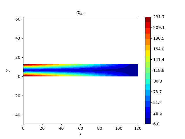
225 # Plot the von Mises stress result using 20 color levels
226 Display.Plot_Result(simu, "Svm", ncolors=20)
227
228 if makeParaview:
229 # Generate Paraview files for visualization
230 Paraview.Save_simu(simu, folder, details=True)
231
232 # Show the total computation time
233 print()
234 Tic.Resume()
235
236 # Display the computation time history
237 # Tic.Plot_History(folder)
238
239 # Show all plots
240 plt.show()
Total running time of the script: (0 minutes 4.215 seconds)