Note
Go to the end to download the full example code.
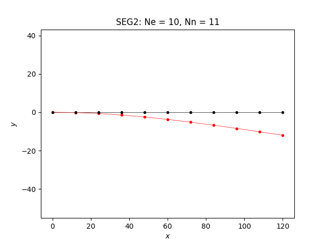
Beam2#
A cantilever beam undergoing bending deformation.
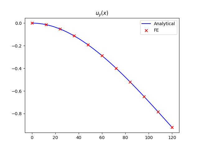
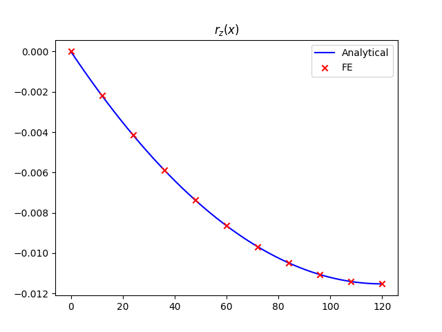
err uy: 1.21e-10 %err rz: 1.12e-10 %
==================== Mesh ====================
Element type: SEG2
Ne = 10, Nn = 11
==================== Model ====================
<EasyFEA.Models.Beam._beam.BeamStructure object at 0x71cb5dda11d0>
solver : scipy
============= Boundary Conditions =============
Unspecified.
=================== Results ===================
Ux max = 0.00e+00
Ux min = 0.00e+00
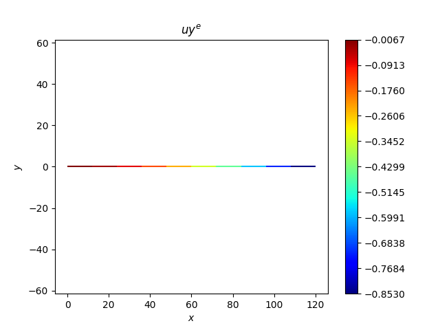
Uy max = 0.00e+00
Uy min = -9.22e-01
=================== TicTac ===================
Mesh : 8.541 ms
Boundary Conditions : 12.875 µs
Matrix : 4.977 ms
Solver : 860.453 µs
Display : 27.753 ms
13 import matplotlib.pyplot as plt
14 import numpy as np
15
16 from EasyFEA import Display, Models, Mesher, ElemType, Simulations
17 from EasyFEA.Geoms import Domain, Line
18
19 if __name__ == "__main__":
20 Display.Clear()
21
22 # ----------------------------------------------
23 # Configuration
24 # ----------------------------------------------
25
26 # geom
27 L = 120
28 nL = 10
29 h = 13
30 b = 13
31
32 # model
33 E = 210000
34 v = 0.3
35
36 # load
37 load = 800
38
39 # ----------------------------------------------
40 # Mesh
41 # ----------------------------------------------
42
43 elemType = ElemType.SEG2
44 beamDim = 2 # must be >= 2
45
46 # Create a section object for the beam mesh
47 mesher = Mesher()
48 section = mesher.Mesh_2D(Domain((0, 0), (b, h)))
49
50 p1 = (0, 0)
51 p2 = (L, 0)
52 line = Line(p1, p2, L / nL)
53 beam = Models.Beam.Isotropic(beamDim, line, section, E, v)
54
55 mesh = mesher.Mesh_Beams([beam], elemType=elemType)
56
57 # ----------------------------------------------
58 # Simulation
59 # ----------------------------------------------
60
61 Iy = beam.Iy
62 Iz = beam.Iz
63
64 # Initialize the beam structure with the defined beam segments
65 beamStructure = Models.Beam.BeamStructure([beam])
66
67 # Create the beam simulation
68 simu = Simulations.Beam(mesh, beamStructure)
69 dof_n = simu.Get_dof_n()
70
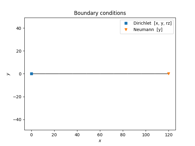
71 # Apply boundary conditions
72 simu.add_dirichlet(mesh.Nodes_Point(p1), [0] * dof_n, simu.Get_unknowns())
73 simu.add_neumann(mesh.Nodes_Point(p2), [-load], ["y"])
74
75 # Solve the beam problem and get displacement results
76 sol = simu.Solve()
77 simu.Save_Iter()
78
79 # ----------------------------------------------
80 # Results
81 # ----------------------------------------------
82
83 Display.Plot_Mesh(simu, deformFactor=-L / 10 / sol.min())
84 Display.Plot_BoundaryConditions(simu)
85 Display.Plot_Result(simu, "uy")
86
87 rz = simu.Result("rz")
88 v = simu.Result("uy")
89
90 x = np.linspace(0, L, 100)
91 uy_x = load / (E * Iz) * (x**3 / 6 - (L * x**2) / 2)
92
93 flecheanalytique = load * L**3 / (3 * E * Iz)
94 err_uy = np.abs(flecheanalytique + v.min()) / flecheanalytique
95 Display.MyPrint(f"err uy: {err_uy * 100:.2e} %")
96
97 # Plot the analytical and finite element solutions for vertical displacement (v)
98 axUy = Display.Init_Axes()
99 axUy.plot(x, uy_x, label="Analytical", c="blue")
100 axUy.scatter(mesh.coord[:, 0], v, label="FE", c="red", marker="x", zorder=2)
101 axUy.set_title("$u_y(x)$")
102 axUy.legend()
103
104 rz_x = load / E / Iz * (x**2 / 2 - L * x)
105 rotalytique = load * L**2 / (2 * E * Iz)
106 err_rz = np.abs(rotalytique + rz.min()) / rotalytique
107 Display.MyPrint(f"err rz: {err_rz * 100:.2e} %")
108
109 # Plot the analytical and finite element solutions for rotation (rz)
110 axRz = Display.Init_Axes()
111 axRz.plot(x, rz_x, label="Analytical", c="blue")
112 axRz.scatter(mesh.coord[:, 0], rz, label="FE", c="red", marker="x", zorder=2)
113 axRz.set_title("$r_z(x)$")
114 axRz.legend()
115
116 print(simu)
117
118 plt.show()
Total running time of the script: (0 minutes 0.245 seconds)