Note
Go to the end to download the full example code.
Beam1#
Beam subjected to pure tensile loading.
Beam: section uses linear TRI3 elements — _Get_shear_correction_factor converges at O(h²). Use TRI6 / QUAD8 (or finer mesh) for accurate k.
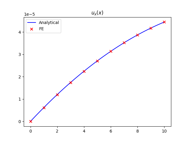
err ux: 1.52e-14%
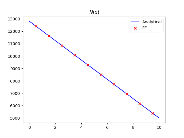
err N: 4.40e-14%
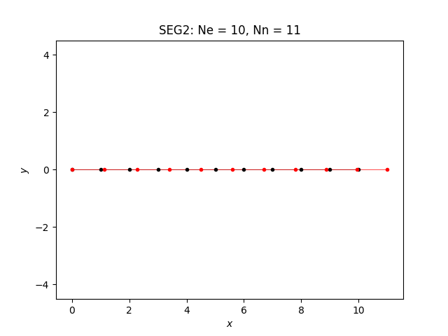
==================== Mesh ====================
Element type: SEG2
Ne = 10, Nn = 11
==================== Model ====================
<EasyFEA.Models.Beam._beam.BeamStructure object at 0x70da16f86590>
solver:scipy
============= Boundary Conditions =============
Unspecified.
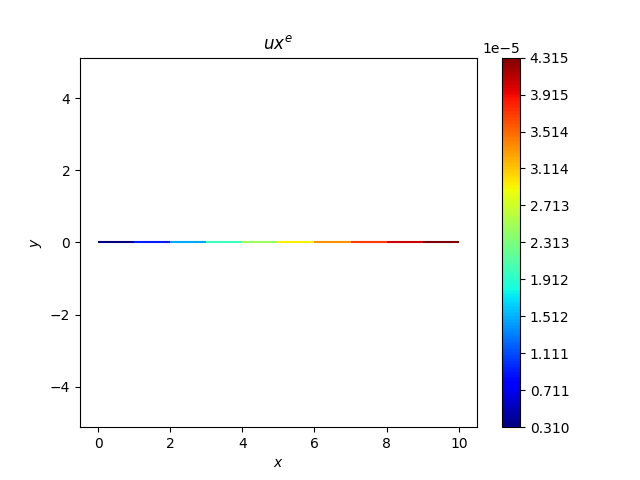
=================== Results ===================
Ux max = 4.45e-05
Ux min = 0.00e+00
=================== TicTac ===================
Mesh: 12.722 ms
Boundary Conditions: 42.677 µs
Matrix: 19.375 ms
Solver: 2.944 ms
Display: 42.357 ms
13 import matplotlib.pyplot as plt
14 import numpy as np
15
16 from EasyFEA import Display, Models, Mesher, ElemType, Simulations
17 from EasyFEA.Geoms import Domain, Line
18
19 if __name__ == "__main__":
20 Display.Clear()
21
22 # ----------------------------------------------
23 # Configuration
24 # ----------------------------------------------
25
26 # geom
27 L = 10
28 nL = 10
29 h = 0.1
30 b = 0.1
31
32 # model
33 E = 200000e6
34 v = 0.3
35 rho = 7800
36 beamDim = 1
37
38 # load
39 g = 10
40 q = rho * g * (h * b)
41 F = 5000
42
43 # ----------------------------------------------
44 # Mesh
45 # ----------------------------------------------
46
47 # Create a section for the beam
48 mesher = Mesher()
49 section = mesher.Mesh_2D(Domain((0, 0), (b, h)))
50
51 p1 = (0, 0)
52 p2 = (L, 0)
53 line = Line(p1, p2, L / nL)
54 beam = Models.Beam.Isotropic(beamDim, line, section, E, v)
55
56 mesh = mesher.Mesh_Beams([beam], elemType=ElemType.SEG2)
57
58 # ----------------------------------------------
59 # Simulation
60 # ----------------------------------------------
61
62 # Initialize the beam structure with the defined beam segments
63 beamStructure = Models.Beam.BeamStructure([beam])
64
65 # Create the beam simulation
66 simu = Simulations.Beam(mesh, beamStructure)
67 dof_n = simu.Get_dof_n()
68
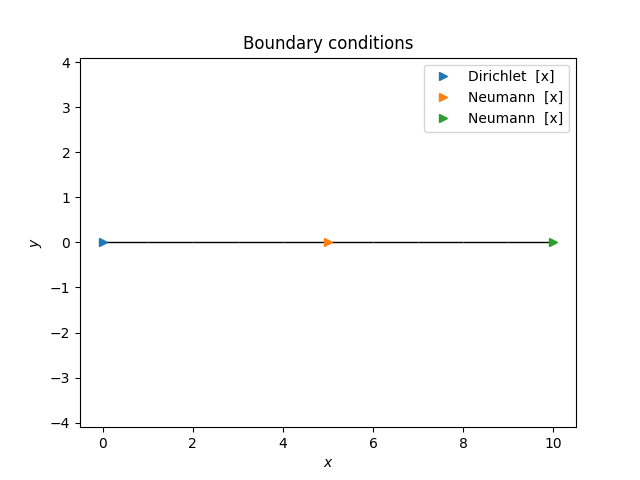
69 # Apply boundary conditions
70 simu.add_dirichlet(mesh.Nodes_Point(p1), [0] * dof_n, simu.Get_unknowns())
71 simu.add_lineLoad(mesh.nodes, [q], ["x"])
72 simu.add_neumann(mesh.Nodes_Point(p2), [F], ["x"])
73
74 # Solve the beam problem and get displacement results
75 sol = simu.Solve()
76 simu.Save_Iter()
77
78 # ----------------------------------------------
79 # Results
80 # ----------------------------------------------
81
82 Display.Plot_Mesh(simu, deformFactor=L / 10 / sol.max())
83 Display.Plot_BoundaryConditions(simu)
84 Display.Plot_Result(simu, "ux")
85
86 # ------------------------
87 # ux
88 # ------------------------
89
90 A = section.area
91 x = np.linspace(0, L, 100)
92 ux_x = lambda x: (F * x / (E * A)) + (rho * g * x / 2 / E * (2 * L - x))
93
94 ux = simu.Result("ux")
95 x_n = mesh.coord[:, 0]
96 err_ux = np.abs(ux_x(x_n) - ux).max() / np.abs(ux_x(L))
97 Display.MyPrint(f"\nerr ux: {err_ux * 100:.2e}%")
98
99 axUx = Display.Init_Axes()
100 axUx.plot(x, ux_x(x), label="Analytical", c="blue")
101 axUx.scatter(x_n, ux, label="FE", c="red", marker="x", zorder=2)
102 axUx.set_title("$u_x(x)$")
103 axUx.legend()
104
105 # ------------------------
106 # N
107 # ------------------------
108
109 N_x = lambda x: F + q * (L - x)
110
111 x_e = x_n[mesh.connect].mean(1) # element centroid x-coords
112 N = simu.Result("N", nodeValues=False)
113 err_N = np.abs(N_x(x_e) - N).max() / np.abs(N_x(x_e)).max()
114 Display.MyPrint(f"\nerr N: {err_N * 100:.2e}%")
115
116 axN = Display.Init_Axes()
117 axN.plot(x, N_x(x), label="Analytical", c="blue")
118 axN.scatter(x_e, N, label="FE", c="red", marker="x", zorder=2)
119 axN.set_title("$N(x)$")
120 axN.legend()
121
122 print(simu)
123
124 plt.show()
Total running time of the script: (0 minutes 0.372 seconds)