Beginner’s Guide

You can follow this guide along with this video.

---

Like any Python script, you should start by importing the core modules from the EasyFEA package:

from EasyFEA import Display, ElemType, Models, Simulations
from EasyFEA.Geoms import Domain

---

The most commonly used modules in EasyFEA are:

Display	Module containing functions used to display simulations and meshes with matplotlib (https://matplotlib.org/).
ElemType(value)	Implemented Lagrange isoparametric element types.
Models	Module implementing constitutive laws used in simulations.
Simulations	This module contains all available simulation classes.
Geoms	Module containing the geometric functions used to build meshes.

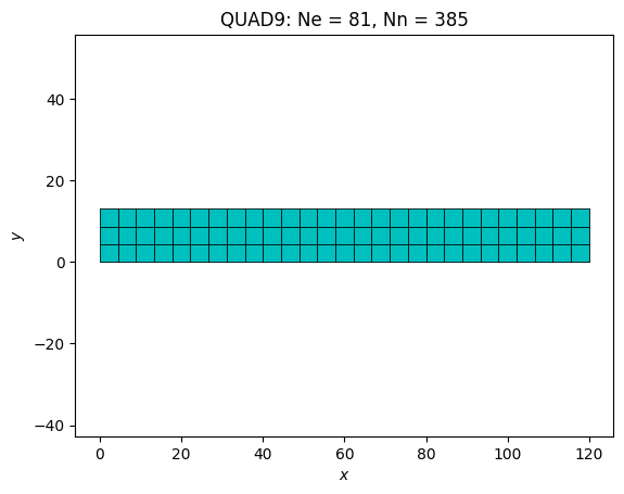
Let’s now create a 2D Mesh using a simple rectangular domain:

# ----------------------------------------------
# Mesh
# ----------------------------------------------
L = 120  # mm
h = 13

domain = Domain((0, 0), (L, h), h / 3)
mesh = domain.Mesh_2D([], ElemType.QUAD9, isOrganised=True)
Display.Plot_Mesh(mesh)

<Axes: title={'center': 'QUAD9: Ne = 81, Nn = 385'}, xlabel='$x$', ylabel='$y$'>

---

Next, define a linear Isotropic material and set up the Elastic simulation:

# ----------------------------------------------
# Simulation
# ----------------------------------------------
E = 210000  # MPa
v = 0.3
F = -800  # N

mat = Models.Elastic.Isotropic(2, E, v, planeStress=True, thickness=h)

simu = Simulations.Elastic(mesh, mat)

---

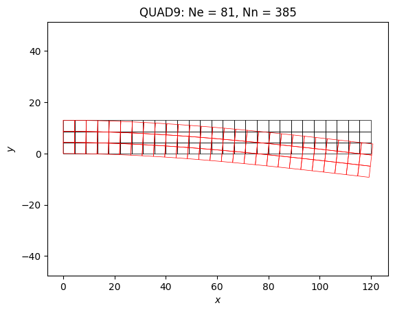
Once the simulation has been set up, defining boundary conditions, solving the problem, and visualizing the results is straightforward.

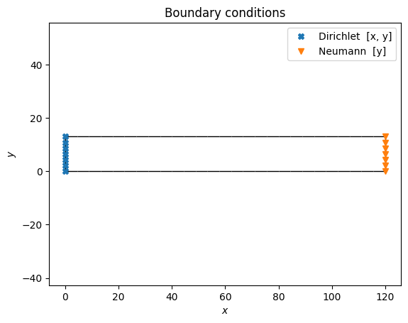
nodesX0 = mesh.Nodes_Conditions(lambda x, y, z: x == 0)
nodesXL = mesh.Nodes_Conditions(lambda x, y, z: x == L)

simu.add_dirichlet(nodesX0, [0, 0], ["x", "y"])
simu.add_surfLoad(nodesXL, [F / h / h], ["y"])

simu.Solve()

# ----------------------------------------------
# Results
# ----------------------------------------------
Display.Plot_Mesh(simu, deformFactor=10)
Display.Plot_BoundaryConditions(simu)
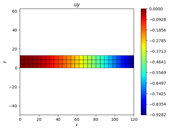
Display.Plot_Result(simu, "uy", plotMesh=True)
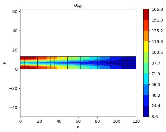
Display.Plot_Result(simu, "Svm", plotMesh=True, ncolors=11)

<Axes: title={'center': '$\\sigma_{vm}$'}, xlabel='$x$', ylabel='$y$'>

---

This script is available in the HelloWorld example.

---

Next steps

I want to …	Guide
Describe a geometry	Create a geometric object
Create a mesh from scratch	Create a mesh
Choose a material model	Create a model
Apply loads and constraints	Apply boundary conditions
Import an external mesh file	Import a mesh
Visualize and export results	Post-process simulation results
Understand what happens inside Solve()	Understand the solve pipeline

For the full list of available simulations and API details, see the examples and API reference.